4.9 Road transport
Road transport is explicitly modelled in WITCH, in two modules representing the passenger (in particular Light Duty Vehicles, LDVs) and the freight sectors. The rest of the transport sector is indirectly modelled in the aggregated non-electric sector in the CES structure.
The LDV types (jveh) represented in the model are:
traditional combustion cars, trad_cars;
hybrid cars, hybrid;
plug-in hybrid cars, plg_hybrid;
electric drive cars, edv.
The same vehicle classification is applied to trucks, jfrt:
traditional combustion trucks, trad_stfr;
hybrid trucks, hbd_stfr;
plug-in hybrid trucks, plg_hbd_stfr;
electric drive trucks, edv_stfr.
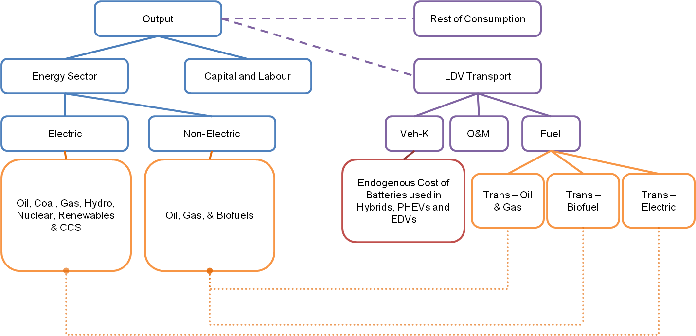
The figure below shows how the structure of the road transport sector fits within WITCH. The composition of vehicle types (denoted in the figure as Veh-K) is determined by a Leontief function of a range of different costs. These comprise the vehicle cost, including battery cost ($/kWh), O&M costs, fuel costs and any associated carbon costs based on the fuel mix within the sector. Fuels are sourced from the Energy sector.
4.9.1 Number of Vehicles
The number of vehicles (both LDV and freight) is set equal to a projection depending on GDP and population growth. This projection is not part of the optimization process (i.e. given GDP and population, demand is given).
Concerning LDVs, the calculation of the number of vehicles per thousand capita \(ldv\_pthc(t,n)\) is based on the IEA/SMP model (Fulton and Eads 2004) which is in turn based on the work of (Dargay and Gately 1999). The following equation has been implemented with parameters set to those in the table below. In particular, the Autonomous Increase (AI) and the Ownership Growth Elasticity (OGE) values depend on the GDP per capita and on the relevant ownership level.
\[ ldv\_pthc(t,n) = ldv\_pthc(t-1,n) \times \left(1+(\frac{gdp\_pc(t,n)}{gdp\_pc(t-1,n)}-1)\times OGE\right)+AI \]
| gdp_pc levels | Maximum ownership level | Ownership Elasticity | Autonomous Increase (AI) |
|---|---|---|---|
| \(\le\) $5000 | no maximum | 0.30 | 3 |
| \(>\) $5000 | 300 vehicles per thousand capita | 1.30 | 3 |
| \(>\) $5000 | 500 vehicles per thousand capita | 0.60 | 3 |
| \(>\) $5000 | 600 vehicles per thousand capita | 0.25 | 4 |
| \(>\) $5000 | n/a | 0.10 | 4 |
The total number of vehicles is obtained by multiplying this value by the population.
\[ ldv\_total(t,n) = ldv\_pthc(t,n) \times population(t,n) \]
Concerning trucks, the total number of vehicles, \(strf\_total\), grows over time according to the GDP per capita growth (again, following the IEA/SMP modelling assumption, Fulton and Eads (2004)).
\[ strf\_total(t,n) = strf\_total(t-1,n) \times \frac{gdp\_pc(t,n)}{gdp\_pc(t-1,n)} \]
The composition of the vehicle fleet, for both LDVs and freight, is then determined by the optimization model, where a linear competition among the vehicle types takes place (mitigated by the presence of additional restrictions and constraints, see below).
\[ ldv\_total(t,n) = \sum_{jveh} K_{EN}(jveh,t,n) \]
\[ strf\_total(t,n) = \sum_{jfrt} K_{EN}(jfrt,t,n) \]
4.9.2 Kilometre Demand and Fuel Consumption
Energy consumption associated to the different vehicle types is given by the product of the number of vehicles, the kilometre demand per vehicle (km_d) and the specific fuel consumption (fuel_cons):
\[ Q_{EN}(jveh,t,n) = km\_d\_ldv(t,n) \times fuel\_cons(jveh,t,n) \times K_{EN}(jveh,t,n) \]
The equation is written for LDVs (jveh), but the same applies to freight (jfrt).
Fuel consumption is the energy consumed by each vehicle for covering one kilometre. It exponentially decreases over time in order to simulate advancements in vehicle efficiency, approximately halving by the end of the century.
\[ fuel\_cons(jveh,t,n) = fuel\_cons\_2005(jveh,n) \times t^{fueleff\_rate(t,n)} \]
Concerning LDVs, the kilometre demand is calculated starting from the travel intensity, derived from IEA/SMP and considered constant over time in the different regions, according to the following scheme:
\[ km\_d\_ldv\_tot(t,n) = travel\_intensity\_ldv(t,n) \times GDP(t,n) \]
\[ km\_d\_ldv(t,n) = \frac{km\_d\_ldv\_tot(t,n)}{ldv\_total(t,n)} \]
Service demand is given by the kilometre demand multiplied by the load factor, i.e. the number of average occupants per vehicle.
\[ s\_d\_ldv(t,n) = load\_factor\_ldv(t,n) \times km\_d\_ldv(t,n) \]
For trucks, the kilometre demand is given and fixed over time. Service demand is again given by the multiplication between the kilometre demand and the load factor, which for trucks is given by the average tonnes of freight carried:
\[ s\_d\_stfr(t,n) = load\_factor\_stfr(t,n) \times km\_d\_stfr(t,n) \]
4.9.3 Cost of Vehicles
While the cost of traditional combustion vehicles is held constant at 2005 levels, the cost of battery integrated vehicles decreases with investments in R&D for batteries. The learning rate is fixed to 12.5%.
An example of how the cost of batteries impacts the cost of vehicles is shown in the following equation for electric LDVs:
\[ veh\_cost(\text{edv},t,n) = {inv\_cost\_trad\_cars \times 0.75 + size\_battery(\text{edv}) \times SC(\text{battery},t,n)} \]
Twenty five percent of the base traditional combustion vehicle cost (inv_cost_trad_cars) is removed so as to allow for the lack of a combustion engine.
The battery size of vehicles is reported in the table below along with the initial cost of vehicles.
| Vehicle type | Battery size (kWh) | Initial vehicle cost (thousand $) |
|---|---|---|
| trad_cars | na | 25 |
| hybrid | 1.5 | 27 |
| plg_hybrid | 13.3 | 44 |
| edv | 75 | 74 |
| trad_stfr | na | 154 |
| hbd_stfr | 8.75 | 165 |
| plg_hbd_stfr | 78.75 | 253 |
| edv_stfr | 262.5 | 445 |
4.9.4 Technology Restrictions and Constraints
Being based on cost considerations not moderated by lower-than-infinite elasticities, one of the main problems with linear competition among technologies is that irregular behaviours might take place, and in particular a sudden switch from one technology to another. Linear models thus normally introduce a set of restrictions or constraints which weaken this effect.
One example is given by the growth curves applied within the model as an endogenous constraint upon the introduction of interim technology options. A logistic functional form is the default, which is defined as follows:
\[ K_{EN}(jinv,t+1,n)-K_{EN}(jinv,t,n) < 1.124 \times \left(1-\frac {K_{EN}(jinv,t,n)}{ldv\_total(t,n)}\right) \times K_{EN}(jinv,t,n) \]
The value of 1.124 has been set using a logistic function fitted to projections of the number of hybrid vehicles for the period between 2010 and 2035 sourced from World Energy Outlook 2010. The equation is applied to both LDVs and trucks.
In addition to an S-shaped diffusion path due to the above function, additional constraints related to the diffusion of technology include:
a limit on the amount of biofuel that can be used in each vehicle (a maximum of 50/50 biofuel/oil mixture is set up to 2020, then linearly increasing up to 100% allowed biofuel share in 2100),
a restriction which constrains investments in a specific vehicle type to at least 30% of what they were in the previous period. Note that this restriction is intended to prevent investments disappearing in a interim technology at too fast a pace.
More details regarding the LDV modelling can be found in (Bosetti and Longden 2013), while the freight sector modelling is described in Carrara and Longden (forthcoming, 2016).