8.1 Economic impacts from climate change

As outlined in the Economy chapter, a set of regional reduced-form damage functions (\(\Omega\)) links the global average temperature increase above pre-industrial levels to changes in regional gross domestic product. Damage functions consist of two components accounting for both negative and positive impacts. Adaptation, \(Q(ADA,t,n)\), reduces the extent to which temperature increase reduces output:

\[ \Omega(t,n) = 1+ \frac{\Big(\omega_{1,n}^-T(t,n) + \omega_{2,n}^-T(t,n)^{\omega_{3,n}^-}+\omega_{4,n}^-\Big)}{1+Q(ADA,t,n)^{\epsilon(n)}} + \Big(\omega_{1,n}^+T(t,n) + \omega_{2,n}^+T(t,n)^{\omega_{3,n}^+}+\omega_{4,n}^+\Big) \]

Economic damages as a percentage of GDP can be computed from \(\Omega(t,n)\) as follows:

\[ Damages(\%\ of\ GDP) = 1 - \frac{1}{\Omega(t,n)} \]

8.1.1 Calibration

The damage functions implemented in the WITCH model are based on sectoral climate impact estimates from the ClimateCost project (Watkiss 2011), described in detail in (Bosello and De Cian 2014), and they are integrated with estimates for the impact categories health and catastrophic events from (Nordhaus 2008). For the category settlements and ecosystems, new estimates are computed using a Willingness-To-Pay approach (see below).

Of the sectors examined by the ClimateCost project, only those overlapping with Nordhaus and Boyer (2000) have been included, namely coastal impacts, energy demand (which is included in the other vulnerable markets category), agriculture, and health for Europe (reduced work capacity due to thermal discomfort). The direct impacts on specific sectors have been evaluated by sectoral models (Brown et al 2011, Vafeidis et al 2008; Mima et al 2011, Criqui 2001, Criqui et al 2009; Iglesias et al 2011; and Kovats and Lloyd 2011, respectively). All estimates, with the exception of health, which are only available for Europe, have been assessed for the thirteen WITCH regions (Chapter 2). Macroeconomic impacts on regional GDP have been calculated for each impact category separately using the computable general equilibrium (CGE) model ICES (Eboli et al 2010, Bosello et al 2012). Therefore, the damage estimates for these three categories include autonomous, or market-driven adaptation. Indirect impact estimates resulting from CGE models are generally smaller than the direct impact estimates from sectoral studies, especially when production factors, such as land or crop yields, are affected. Input substitution makes it possible to buffer the direct impacts. Input substitution interacts with terms of trade effect, differentiating the resulting indirect impacts from direct impacts from bottom-up models quite significantly.

Impacts have been estimated for a temperature increase above pre-industrial levels of 1.9 degree Celsius and they have been extended to other temperature increases, including the calibration point 2.5 degree Celsius, using sector specific assumptions. For the categories coastal impacts and agriculture we use a power relationship as in Nordhaus and Boyer (2000). We assume that for warming above 3 degree Celsius all regions begin to lose, following the evidence that crop productivities decline in all regions for such a threshold. Energy and health impacts have been extended using a linear trend. Catastrophic impacts are interpolated using a linear function up to the temperature increase of 3 degree Celsius above pre-industrial levels, and using a quadratic equation above that threshold. Below we briefly summarize how impacts have been estimated in each impact category. More details can be found in (Bosello and De Cian 2014).

Agriculture. Changes in the average productivity of crops are from the ClimateCrop model (Iglesias et al. 2011). Crop response depends on temperature. CO2 fertilisation and extreme events, and water management practices are also taken into account. Spatially integrating all these elements, the ClimateCrop model estimates climate change impacts and the effect of the implementation of different adaptation strategies.

Coastal. Estimates of coastal land loss due to sea-level rise (Brown et al 2011) are from the Dynamic Integrated Vulnerability Assessment (DIVA) model (Vafeidis et al 2008). DIVA is an engineering model designed to study the vulnerability of coastal areas to the rise in sea-level. The model is based on a world database of natural system and socio-economic factors for world coastal areas. Changes in natural as well as socio-economic conditions of possible future scenarios are implemented through a set of impact-adaptation algorithms. Impacts are then assessed both in physical (i.e. sq. km of land lost) and economic (i.e. value of land lost and adaptation costs) terms.

Health. This category refers to damages due to malaria, dengue, tropical diseases and pollution. Impact estimates are from Nordhaus (2007). For Europe, impacts also include damages on labour productivity estimated by Kovats and Lloyd (2011). They assess the change in working conditions due to heat stress produced by the increase in temperature, and they estimate the expected decrease in labour productivity for four European macro-regions (Western, Eastern, Northern and Southern).

Settlements and ecosystems. WITCH estimates rely on a Willingness-To-Pay (WTP) approach, as in Nordhaus and Boyer (2000). Those estimates have been replaced with updated calculations of the WTP following the approach used in the MERGE model (Manne and Richels, 2005). In MERGE, the WTP to avoid the non-market damages of a 2.5 degree Celsius temperature increase above pre-industrial levels is 2% of GDP when per capita income reaches 40,000 USD 1990. The 2% figure was the US EPA expenditure on environmental protection in 1995. A s-shaped relationship between per capita income and WTP is then used to infer the WTP for other regions. WITCH follows a similar approach, but using an updated proxy for the WTP, considering the EU expenditure on environmental protection. The most recent Eurostat data (Environmental Protection Expenditure in Europe by public sector and specialized producers 1995-2002) referring to public sector expenditure reports a total value in 2001 of 54 billion EUR, 0.6% of EU25 GDP, or of 120 EUR per capita. This value covers activities such as protection of soil and groundwater, biodiversity and landscape, noise protection, radiation, along with more general research and development, administration and multifunctional activities. We then use the expression reported in Warren et al. (2006), which links average per capita environmental expenditure and per capita income to extrapolate a relationship between WTP and per-capita income. The s-shaped relationship between per-capita income and WTP has been used to compute the WTP in the different model regions. The resulting estimates fall between Nordhaus and Boyer (2000) and MERGE estimates as described in Warren et al. (2006). The WTP reference value used for rich countries crucially determines the final results . Using the EU values as the benchmark for calculations yields lower damages than in the MERGE model, but higher than Nordhaus and Boyer (2000). A WTP approach tends to produce higher evaluations for non-market ecosystem losses in high-income countries, although ecosystem/biodiversity richness is highly concentrated in developing countries.

Other vulnerable markets. This category refers to the effect of climate change on energy. WITCH uses the change in residential energy demand due to increasing temperatures derived from the POLES model (Mima et al. 2011, Criqui 2001, Criqui et al. 2009). POLES is a bottom-up partial-equilibrium model of the world energy system extended to include information on water resource availability and adaptation measures. It determines future energy demand and supply according to energy price trends, technological innovation, climate impacts and alternative mitigation policy schemes. The model considers both heating and cooling degree-days in order to determine the evolution of demand for different energy sources (coal, oil, natural gas, electricity) over the time-horizon considered.

Catastrophic. This category refers to the willingness to pay to avoid catastrophic events, and it is based on Nordhaus (2007).

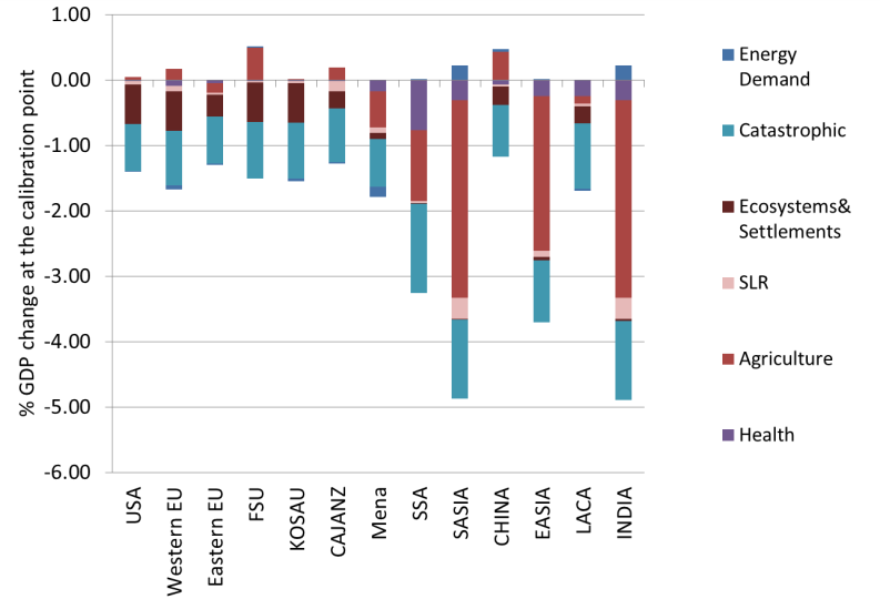
Figure 8.1 below decomposes regional climate impacts at the calibration point (2.5 degree Celsius global average temperature increase above pre-industrial levels) by impact category.

Climate change impacts at calibration point when global average temperature increases 2.5 degree Celsius above pre-industrial levels.

References

Bosello, F., and E. De Cian. 2014. “Documentation on the Development of Damage Functions and Adaptation in the WITCH Model.” RP0228. Fondazione Centro Euro-Mediterraneo sui Cambiamenti Climatici.

Nordhaus, William. 2008. A Question of Balance: Weighing the Options on Global Warming Policies. Yale University Press.