Energy supply
WITCH includes a comprehensive range of technology options to
describe the final use of energy and the generation of electricity.
The energy sector is described by a production function that aggregates
different factors at various levels and with associated elasticities of substitution \(\rho\).
The main distinction is among electric generation and non-electric
consumption of energy.
The key technological-economic features represented are:
yearly utilisation factors, fuel efficiencies, investment, and
operation and maintenance costs, capital depreciation.
The following graph shows the fundamental CES nest structure of the economy and energy system. The number below a node represents the elasticity of substitution at a given nested CES.
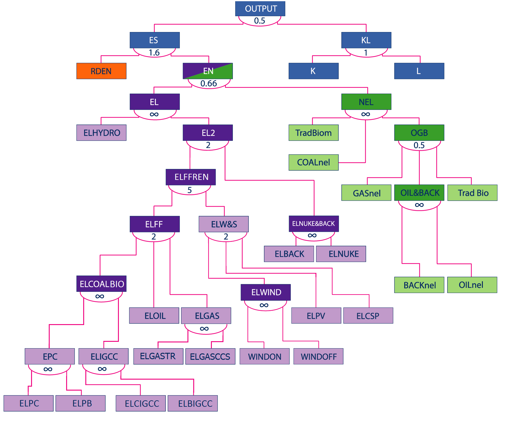
CES Production Function of WITCH
Electric energy technology sectors
Electricity is generated by a series of traditional fossil fuel-based
technologies and carbon-free options.
Fossil fuel-based technologies include natural gas combined cycle (NGCC),
fuel oil and pulverised coal (PC) power plants.
Coal-based and Biomass-based electricity can also be generated using integrated gasification combined cycle (IGCC) production with carbon capture and storage (CCS). Other CCS technologies are coal post-combustion, coal oxyfuel plants, NGCC with carbon capture and retrofitting unit for existing coal plants.
Low carbon technologies include hydroelectric and nuclear power, renewable sources such as wind turbines and photovoltaic panels and CSP (wind and solar), and two carbon-free backstop technologies, which represent a basket of technological options far from commercialization.
The cost of electricity generation is endogenous and combines capital costs, O&M expenditure, and the costs for fuels.
For nuclear power, waste management costs are also modelled, but no exogenous constraint is assumed.
The following table provides a full list of the CES nodes including all energy options:
| KL |
Capital-labor aggregate |
ELNUKE&BACK |
Electricity generated with nuclear and backstop |
| K |
Capital invested in the production of the final good |
ELBACK |
Electricity generated with backstop |
| L |
Labor |
ELNUKE |
Electricity generated with nuclear |
| ES |
Energy services |
ELW&S |
Wind turbines and photovoltaic panels |
| RDEN |
Energy R&D capital |
NEL |
Nonelectric energy |
| EN |
Energy |
TradBiom |
Traditional Biomass |
| EL |
Electric energy |
COALnel |
Coal for nonelectric energy |
| ELYHYDRO |
Electricity generated with hydroelectric |
OGB |
Oil, backstop, gas, and biofuel |
| EL2 |
Electricity generation |
GASnel |
Gas for nonelectric energy |
| ELFF |
Fossil fuel electricity |
OIL&BACK |
Oil and backstop for nonelectric energy |
| ELCOALBIO |
Electricity generated with Coal and Biomass |
BACKnel |
Backstop for nonelectric energy |
| EPC |
Electricity generated with pulverized coal |
OILnel |
Oil for nonelectric energy |
| ELIGCC |
Electricity generated with integrated gasification combined cycle coal plus carbon capture and storage |
Biofuels |
Traditional and advanced biofuels |
| ELOIL |
Electricity generated with oil |
Trad Bio |
Traditional biofuels |
| ELGAS |
Electricity generated with gas |
ELWIND |
Electricity generated with Wind Energy |
| ELGASTR |
Electricity generated with Gas turbines |
ELPV |
Electricity generated with Photovoltaics |
| ELGASCCS |
Electricity generated with Gas with CCS |
ELCSP |
Electricity generated with Concentrated Solar Power |
| WINDON |
Electricity generated with Onshore Wind |
WINDOFF |
Electricity generated with Offshore Wind |
| ELPC |
Electricity generated with Pulverised Coal |
ELCIGCC |
Electricity generated with Coal IGCC plus CCS |
| ELPC_POST |
Electricity generated with Coal with post-combustion CCS |
ELPC_OXY |
Electricity generated with Coal oxyfuel with CCS |
| ELPB |
Electricity generated with biomass |
ELBIGCC |
Electricity generated with Biomass with CCS |
Capital accumulation for electric energy technology sectors
The capital of some electricity production technologies accumulates as follows:
\[
K_j(t+1,n) = K_j(t,n)\left(1-\delta_j(t+1,n)\right)^{\Delta_t} +
\Delta_t \times \frac{I_j(t,n)}{SC_j(t,n)}, \forall j\in \mathcal{J}_{inv},
\]
where \(\mathcal{J}_{inv}\) is the set of electric energy technology sectors in which one can invest.
For less mature technologies, endogenous technical change is modelled: On the one hand, the investment cost \(SC\) for solar and wind energy is decreasing with the world cumulative installed capacity by means of Learning-by-Doing.
On the other hand, the investment costs \(SC\) for backstop technologies are computed using a Two Factor Learning Curve: costs reductions are driven by both, growth in cumulated installed capacity and accumulation of R&D knowledge.
The aforementioned methodology is shown in the Research and Development section.
Since we use a standard exponential depreciation rule as for the general economy-wide investment, this implies a depreciation of capital which does not exactly replicate the actual lifetime and capacity of a power plant. Therefore, we recalibrate the depreciation rate \(\delta_j(t,n)\) based on a finite lifetime of the power plant.
Based on the lifetimes of the different types of power plants, we assume that the capital depreciates linearly at a rate of 1% p.a. until it reaches its end of life, and is decomissioned afterwards. Based on this more realistic depreciation schedule, we impute an exponential depreciation rate that yields the same life time capacity, i.e., the area under the capacity or capital curve over time, as this depreciation schedule.
The lifetime in years for the different types of energy technology are given in the following table:
| wind |
30 |
| nuclear |
40 |
| hydro,elback |
45 |
| coal |
40 |
| oil |
25 |
| gas |
25 |
| biomass |
25 |
| solar |
22 |
| storage |
22 |
| vehicles |
22 |
The exponential depreciation rate \(\delta_j(t,n)\) can then be computed by equalizing the area under the (right trapezoid) depreciation schedule with the exponential one solving the equation
\[
\intop_{0}^{\infty}e^{-\delta_{j}(t,n)t}dt=\left(1-\frac{1}{2}\cdot0.01\cdot lifetime(j)\right)lifetime(j)
\]
for \(\delta_j(t,n)\). It can be computed as
\[
\delta_j(t,n) = \frac{1}{lifetime(j)-\frac{0.01}{2}*lifetime(j)^2}
\]
which, for instance, yields for a coal fired powerplant with a lifetime of 40 years an exponential depreciation rate of \(\delta_j(t,n)=0.03125\).
Production in electric sector
The structure of WITCH in the figure above is represented by the following CES production functions. As above, the value shares \(\alpha\), efficiency parameters \(\phi\), and substitution parameter \(\rho\) are obtained from the Static Calibration of the model.
The tree for the power sector is defined by the three following equations combining electricity from fossil fuels \(ELFF\), nuclear and the electrical backstop \(EL_nucback\), and intermittent renewable \(EL_intren\) with hydro power \(EL_hydro\) to electricity \(EL(t,n)\):
\[
EL(t,n) = EL2(t,n) + \alpha_{el_{hydro}}(n) EL_{hydro}(t,n)
\]
\[
EL2(t,n) = \phi_{el2}(n) \left(
\alpha_{el2}(n) ELFF(t,n)^{\rho_{el2}(n)} +
\beta_{el2}(n) EL_{nucback}(t,n)^{\rho_{el2}(n)} +
\gamma_{el2}(n) EL_{intren}(t,n)^{\rho_{el2}(n)}
\right)^{\frac{1}{\rho_{el2}}(n)}
\]
\[
ELFF(t,n) = \phi_{elff}(n) \left(
\alpha_{elff}(n) EL_{coalwbio}(t,n)^{\rho_{elff}(n)} +
\beta_{elff}(n) EL_{oil}(t,n)^{\rho_{elff}(n)} +
\gamma_{elff}(n) EL_{gas}(t,n)^{\rho_{elff}(n)}
\right)^{\frac{1}{\rho_{elff}}(n)}
\]
Additional constraints in the electric sector
In the electric sector, the production capacity is bounded by the capital stock times the capacity factor \(\mu\) (mu):
\[
EL_j(t,n) \le \mu_j(t,n) \times KEL_j(t,n)
\]
For sectors that have are fuel fed, the production capacity, \(Q_j\), is equal to the energy consumed times the overall efficiency rate of the sector \(\xi\):
\[
Q_j(t,n) = \sum_f \xi_{j,f}(t,n) \times Q_{j,f}(t,n)
\]
For the backstop technology in the electric sector (advanced nuclear), while Research and Development brings down the future costs (see above), the penetration is limited to 5% of total energy demand in the respective sector per period: \(EL_{elback}\), is bounded by the coefficient lim_elback = 5%.
\[
EL_{elback}(t+1,n) - EL_{elback}(t,n) \le lim\_elback \times \left( EL(t,n) - EL_{elback}(t,n) \right)
\]
Non-electric energy sectors
Energy consumption in the non-electric sector is based on traditional fuels
(traditional biomass, oil, gas and coal) and bio-fuels. This sector comprises
transportation, industrial, and residential and commercial energy use.
The road transport sector is separated out from the CES structure and is described in detail in the section Road Transport (mod_road_transport). The stationary sector comprising industrial, commercial, and residential use of fuels is
defined through a CES nest. It combines non-electric energy use from coal \(NEL_coal\), traditional biomass in developing countries \((NEL_trbiomass)\), and an aggregate of Oil&Gas (and traditional biofuels) use \((NEL_log)\). This CES nest is thus defined by the following two equations, where the CES parameters are as before calibrated in the Static Calibration:
\[
NEL(t,n) = \alpha_{nel_{coal}} NEL_{coal}(t,n) +
NEL_{log}(t,n) +
\alpha_{nel_{trbiomass}} NEL_{trbiomass}(t,n)
\]
The \((NEL_log)\) aggregate combines Oil, Gas, and traditional biofuel which are rather easy substitutable in a separate CES nest:
\[
NEL_{log}(t,n) = \phi_{nelog}(n) \left(
\alpha_{nelog}(n) NEL_{oilback}(t,n)^{\rho_{nelog}(n)} +
\beta_{nelog}(n) NEL_{gas}(t,n)^{\rho_{nelog}(n)} +
\gamma_{nelog}(n) NEL_{trbiofuel}(t,n)^{\rho_{nelog}(n)}
\right)^{\frac{1}{\rho_{nelog}}(n)}
\]
Primary Energy Supply of Fuels
The total primary energy supply of the different fuels is the sum of the consumption from all the sectors:
\[
Q_f(t,n) = \sum_j Q_{j,f}(t,n)
\]
The consumption of fuel \(f\), \(Q_f\), equals the total level of extraction by balancing domestic extraction and fuel imports
\(X_{f}\):
\[
\sum_n Q_f(t,n) = \sum_n X_f(t,n)
\]
If the country is a net exporter, \(X_f\) is negative. The net cost of the different fuels is equal to the cost of extracted fuels consumed fuels minus the cost of the (net-)imported fuels at the world market price \(p_f(t)\)
\[
C_f(t,n) = MC_f(t,n) \times Q_f(t,n) -
p_f(t) \times X_f(t,n)
\]
The price of fossil fuels and exhaustible resources (\(f\), oil, gas, coal and uranium) is determined by the marginal cost of
extraction, \(MC_f\), which in turn depends on current and cumulative extraction. A regional mark-up is added to mimic different regional costs including transportation costs.