2.2 Model scope
2.2.1 Energy Sector
The energy sector is fully integrated with the rest of the economy. It is distinguished in an electric sector, a transportation sector, and an aggregated non-electric (industry, services and residential) sectors.
The primary and secondary forms of energy are:
| Primary Energy | Secondary Energy |
|---|---|
| Coal | Electricity |
| Oil | |
| Gas | |
| Uranium | |
| Bioenergy |
The following power plant technologies are included:
| Power plant |
|---|
| Coal with and without CCS |
| Oil without CCS |
| Gas with and without CCS |
| Wind onshore and offshore |
| Solar PV and CSP |
| Nuclear LWR and advanced |
| Bioenergy with and without CCS |
| Hydro power |
Technologies that are subject to endogenous technological change are: advanced biomass and advanced nuclear. Overall energy efficiency is also subject to endogenous technical change. Moreover, learning-by-doing is taken into account for wind and solar energy.
2.2.2 Land Use Sector
The land use sector is represented in the WITCH model through a soft-linkage with the GLOBIOM land use and forestry model. GLOBIOM is emulated via a response function obtained from a large number of scenarios generated varying the price of biomass (both residues and plantations) and the price of carbon emission from land-use and agriculture. GLOBIOM also provides to WITCH the quantity of available biomass, the CO2 emissions from deforestation and afforestation, the CH4 and N2O emissions from agriculture.
2.2.3 Greenhouse gases and air pollutants
The model computes many emissions species, either endogenously, or based on exogenous assumptions. Mitigation of these emissions is possible through transformation in the energy system, energy efficiency improvements, substitution of fossil fuels, the use of Carbon Capture and Storage (CCS), and land use change. Moreover, for certain emissions, direct abatement is modelled through Marginal Abatement Cost (MAC) curves, or end of pipe measures via emission factors.
| Emissions | Source | Mitigation |
|---|---|---|
| CO2 | Endogenous | see text |
| CH4 | Partially endogenous | Substitution/MAC |
| N2O | Partially endogenous | Substitution/MAC |
| F-gases | Exogenous | MAC |
| SO2 | Partially endogenous | Emissions factors |
| VOC | Partially endogenous | Emissions factors |
| NOx | Partially endogenous | Emissions factors |
| BC | Partially endogenous | Emissions factors |
| OC | Partially endogenous | Emissions factors |
| CO | Partially endogenous | Emissions factors |
| NH3 | Exogenous | RCP database |
2.2.4 Regions
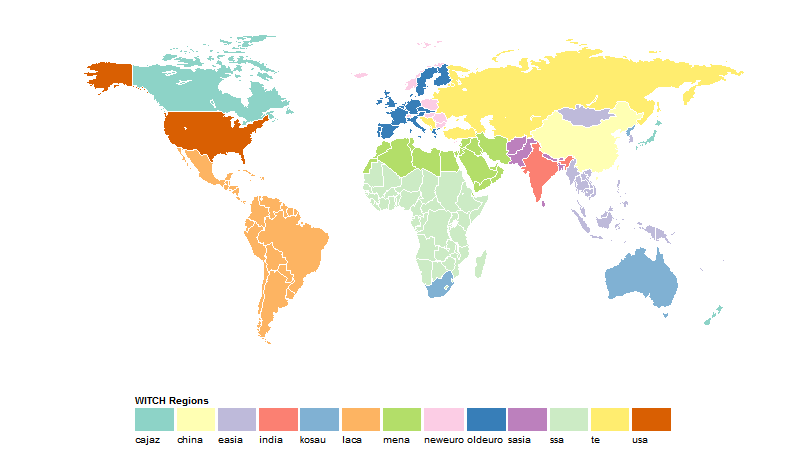
The original version of the model has 13 regions consistent on the basis of geography, income and the structure of energy demand.

WITCH original regions
The following table describes the regional compositions.
| Region Name | Countries |
|---|---|
| cajaz | Canada, Japan, New Zeland |
| china | China and Taiwan |
| easia | South East Asia, including Indonesia |
| india | India |
| kosau | South Korea, South Africa, Australia |
| laca | Latin America, Mexico and Caribbean |
| mena | Middle East and North Africa |
| neweuro | EU new countries |
| oldeuro | EU old countries (EU-15) + EFTA |
| sasia | South Asia (excluding India) |
| ssa | Sub Saharan Africa |
| te | Non-EU Eastern European countries, including Russia |
| usa | United States of America |
2.2.5 Coalitions
The regions of WITCH a priori solver their respective optimization program by default. However, any set of regions cooperating can be modelled as a coalition, which then in turn maximizes the sum of welfare of their members. Two important special cases of coalitions are already defined:
no-cooperation : each region is mapped to a coalition containing only this region. This is the default setting.
full-cooperation: the Grand Coalition containing all world regions.
Coalitions and regions interact with each other because of the presence of economic (technology, exhaustible natural resources) and environmental global externalities.
For each coalition, a forward-looking representative agent maximizes her own inter-temporal social welfare function, strategically and simultaneously to other regions.
The inter-temporal equilibrium is calculated as an open-loop Nash equilibrium. Through the optimization process, regions choose the optimal dynamic path of a set of control variables, namely investments in various technologies. The oil market price, global temperature increase, and emission permits market price–if a cap and trade system is being modelled–are the outcome of the regional strategies and are iteratively solved until the equilibrium is achieved.
2.2.6 Time horizon
The base year of WITCH is 2005 and all economic values are expressed in USD of 2005. The time horizon is 150 years, modelled in 30 periods of 5-year time steps and we denote by \(\Delta_{\text{t}}=5\) the duration of one time step in years. Longer time horizon can also be run until 2300 to avoid any end-of-horizon effect, but 2150 is generally sufficient. Results are usually reported for the period 2005-2100. The periods 2005, 2010 and 2015 are calibrated to the energy and economic historical statistics where available.