8.2 Adaptation
At the core of the adaptation module introduced in the WITCH model there are three control variables that broadly represent various possible adaptive responses, namely building specific adaptive capacity, proactive adaptation, and reactive adaptation, see Figure 8.2.
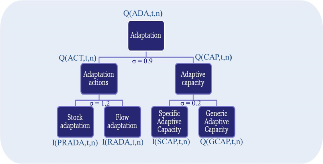
Adaptation at the top nest of the adaptation tree, denoted by the variable \(Q(ADA,t,n)\), reduces the extent to which temperature increase affects output:
\[ \Omega(t,n) = 1+ \frac{\Big(\omega_{1,n}^-T(t,n) + \omega_{2,n}^-T(t,n)^{\omega_{3,n}^-}+\omega_{4,n}^-\Big)}{1+Q(ADA,t,n)^{\epsilon(n)}} + \Big(\omega_{1,n}^+T(t,n) + \omega_{2,n}^+T(t,n)^{\omega_{3,n}^+}+\omega_{4,n}^+\Big) \]
Adaptation combines activities (ACT) and capacity (CAP) to produce adaptation services:
\[ Q(ADA,t,n)= (\omega_{act(n)}Q(ACT,t,n)^{\rho_{ada}}+ (1-\omega_{act(n)})Q(CAP,t,n)^{\rho_{ada}})^{\frac{1}{\rho_{ada}}} \]
Adaptation activities can take the form of reactive adaptation (RADA) and proactive adaptation (PRADA):
\[ Q(ACT,t,n)= \omega_{eff(n)}(\omega_{rada(n)}I(RADA,t,n)^{\rho_{act}}+ (1-\omega_{rada(n)})K(PRADA,t,n)^{\rho_{act}})^{\frac{1}{\rho_{act}}} \]
Proactive adaptation describes measures requiring a stock of defensive capital to be operational before damage materializes, such as the construction of dikes. Reactive adaptation are actions implemented right after climatic impacts effectively occur for the purpose of dealing with any residual damages that anticipatory adaptation or mitigation has been unable to obviate. Examples of these strategies include change in the use of air conditioning or hospitalization and use of health services
Adaptation capacity depends on generic capacity (GCAP) and specific capacity (SCAP) based on a CES function with calibrated share values \(\omega_{gcap(n)\) and can be written this way:
\[ Q(CAP,t,n)= \omega_{eff(n)}(\omega_{gcap(n)}Q(GCAP,t,n)^{\rho_{cap}}+ (1-\omega_{gcap(n)})K(SCAP,t,n)^{\rho_{cap}})^{\frac{1}{\rho_{cap}}} \]
Generic capacity is exogenous and grows at the growth rate of total factor productivity, \(tfp_y(t,n)\). The initial level is given by the 2005 average stock of knowledge (R&D) and human capital (EDU):
\[ Q(GCAP,t,n)= \frac{k0(R\&D,n)+k0(EDU,n)}{2}tfp_y(t,n) \]
The human capital and R&D stock are exogenous and have been computed using the expenditure in total R&D (or education) from the World Development Indicators (2008). The R&D stock is not linked to the energy R&D investments, which instead are endogenous.
Specific adaptive capacity accounts for the investments dedicated to facilitate adaptation activities, such as improvement of meteorological services, early warning systems, the development of climate modelling and impact assessments. Specific capacity and proactive adaptation are stocks that accumulate following the standard perpetual rule:
\[ K(SCAP,t,n+1) = K(SCAP,t,n+1)(1-\delta_{SCAP})^{\Delta_{\text{t}}} +\Delta_{\text{t}} I(SCAP,t,n) \]
\[ K(PRADA,t,n+1) = K(PRADA,t,n+1)(1-\delta_{PRADA})^{\Delta_{\text{t}}} + \Delta_{\text{t}} I(PRADA,t,n) \]
The depreciation rate for proactive adaptation (\(\delta_{PRADA}\)) is 10% and the depreciation rate for specific adaptive capacity is 3%. All forms of adaptation expenditure reduce the resources available for other uses and are subtracted from the budget constraint, see the chapter Economy.
Table 8.1 defines the main variables of the adaptation module.
| Symbol | Definition | GAMS | Unit |
|---|---|---|---|
| \(I_{PRADA}(t,n)\) | Investment in proactive adaptation | I(‘PRADA’,t,n) | T$ |
| \(I_{SCAP}(t,n)\) | Investment in specific ad. capacity | I(‘SCAP’,t,n) | T$ |
| \(I_{RADA}(t,n)\) | Investment in active adaptation | I(‘RADA’,t,n) | T$ |
8.2.1 Calibration of adaptation costs
The WITCH model uses relevant literature supplemented with ad hoc assumptions to estimate the optimal levels of adaptation and its effectiveness. For each impact category, regional data on costs and benefits of adaptation possibilities are collected and used to calibrate the parameters of the adaptation functions used in the model. The calibration process of adaptation costs is described in detail in (Agrawala et al. 2011) and has been updated in (Bosello and De Cian 2014). Costs of adaptation actions and their effectiveness in the sectors considered in the reduced-form damage function have been collected and grouped into three categories of proactive, reactive, and specific capacity.
For the following impact categories only proactive adaptation measures are considered:
Agriculture. WITCH assumes that the most significant cost component of climate change adaptation in agriculture is related to irrigation and water conservation practices, and therefore models adaptation in agriculture as a proactive strategy. The main data source is (UNFCCC 2007), which reports estimates of the future total cost on water infrastructure in a climate change scenario (B1 SRES scenario), assuming that 25% of those investments will be climate change driven. As in (Agrawala et al. 2010) and (Agrawala et al. 2011), we assume that the agricultural sector absorbs 70% of the water infrastructure costs reported by the UNFCCC study, and that 15% (see Agrawala et al. 2010 for a discussion) of these will be necessary in the future for adapting to climate change. Assumptions about adaptation effectiveness follow Agrawala et al. (2011).
Coastal. WITCH model uses estimates from the DIVA model as described in (Agrawala et al. 2010) and (Agrawala et al. 2011).
Settlements and ecosystems. For the ecosystem category, WITCH uses the (UNFCCC 2007) study to revise adaptation costs. We use the observed expenditure on conservation of protected areas (PAs) as a proxy of investments needed to protect natural ecosystems. The global value reported is $7 billion. UNFCCC (2007) estimates an annual increase in expenditure to increase protected areas by 10% up to $12-22 billion in 2030. That range refers to the estimated cost of improving protection, expanding the network of protected areas, and compensating local communities that currently depend on resources from fragile ecosystems. We scaled up the estimated range $12-22 billion to 2050 linearly using the ratio of temperature increase in 2060 relative to the temperature increase in 2030 in the WITCH model (to $21-38 billion), and compute a lower and higher bound for adaptation costs. In this study we use the lowest estimate. The global estimated adaptation costs are allocated to the different regions proportionally to the damage in the ecosystems category.
To estimate adaptation costs in the settlements category we apply the methodology described in (UNFCCC 2007) to the model investments in physical capital in 2060. According to that study, the average annual share of infrastructure vulnerable to the impacts of climate change is 2.7% of average annual investments in infrastructure globally. The World Bank (2006 2011) estimates the additional costs of adapting vulnerable infrastructure to climate change between 5% and 20% of investments. We consider the rate of 5%. The expenditure needed to eliminate the infrastructure gap identified in (Parry, N. Arnell, and Nicholls. 2009) is assumed to be zero for developed countries, and it is included in the specific capacity category. We use aggregate figures for low and middle income countries provided by (Parry, N. Arnell, and Nicholls. 2009) in Table 6.1 to compute the average annual regional investments needed to address the infrastructure adaptation deficit. Assumptions about adaptation effectiveness follow Agrawala et al. (2011).
For the following impact categories only reactive adaptation measures are considered:
Other vulnerable markets (energy). Follow (Agrawala et al. 2010) and (Agrawala et al. 2011), we use adaptation costs related to changes in heating and cooling expenditure from De Cian et al. (2013), an econometric study that estimates the elasticity of electricity, natural gas, coal and oil products to temperature changes by using panel data. With respect to effectiveness, it is assumed that in developed countries the protection level is quite high, 80%, while it is 40% in developing countries, as in (Agrawala et al. 2010) and (Agrawala et al. 2011).
Health. WITCH assumes that adaptation in the health sector is reactive, and cost estimates are from (Tol RSJ 2001), as in (Agrawala et al. 2010) and (Agrawala et al. 2011). Tol and Dowlatabadi (2001) assess the treatment cost associated with climate-driven malaria, dengue, schistosomiasis, diarrhoeal, cardiovascular and respiratory diseases, for different scenarios of temperature increases on a global scale. The effectiveness of adaptation is based on a survey of the literature, which shows that protection levels range between 20% in Africa and 40% in other non-OECD countries. In developed regions protection levels are much higher, ranging from 60% to 90%. The WITCH model relies on the assumptions described in Agrawala et al. (2011).
Catastrophic. As the events considered in this category are large-impact events and catastrophes, the potential to reduce their impacts through adaptation is assumed to be small. Therefore, both protection costs and protection levels are assumed to be small. The costs to address catastrophic events through early warning systems are based on (Agrawala et al. 2010) and (Agrawala et al. 2011), and are considered part of specific capacity. Protection levels are also assumed to be very low, 10% in developed countries and 0.10% in developed countries).
Specific capacity includes:
Expenditure needed to eliminate the infrastructure gap identified in (Parry, N. Arnell, and Nicholls. 2009). It is assumed to be zero in developed countries.
Expenditure needed to empower women through education (Brian et al. 2010)
Early warning systems (Adams, Houston, and McCarl 2000)
R&D expenditure in the agriculture sector (UNFCCC 2007)
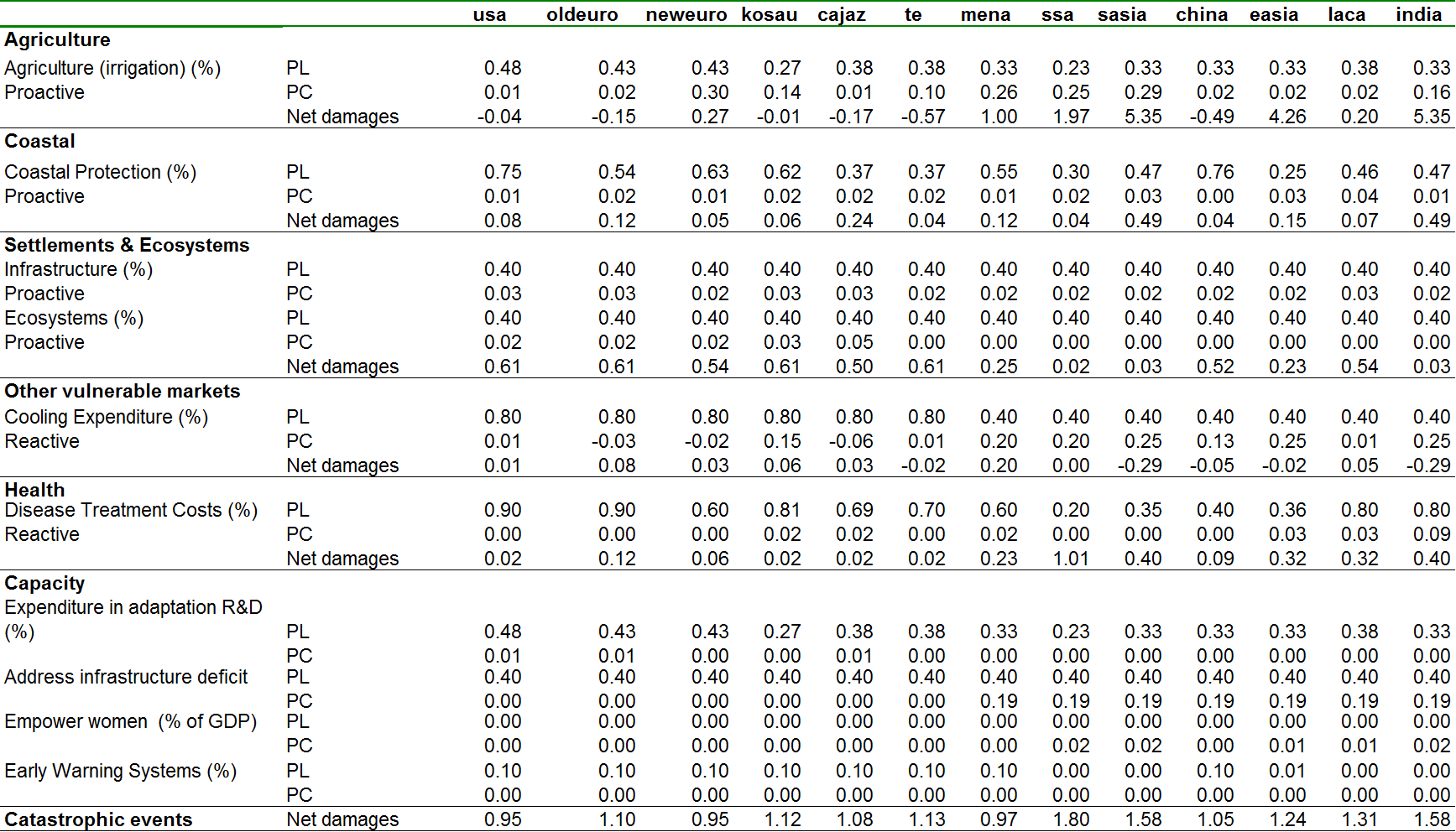
Table 8.3 summarize adaptation costs (PC), protection levels (PL), and net damages at the calibration point when temperature increases by 2.5 degree Celsius above pre-industrial levels.