5.2 Coal and Gas: extraction and trade
The Coal and Gas module introduces extraction for these fuels. Trade (net import of these two fossil fuels) emerges as the ex-post difference between consumption and fossil fuel extraction.
5.2.1 Fossil fuel availability curves
Extraction of coal and gas is modelled by means of fossil fuel availability curves, which define the relationship between cumulative extraction and the cost of producing fossil fuels. In fact, under the hypothesis of perfect competition in the markets, marginal costs equal fuel price, and therefore it is possible to determine the optimal amount of cumulative extraction at the regional level \(cum\_prodpp(f,t,n)\), associated to the international price \(p_f(t)\).
Annual production of fossils is given by the difference between cumulative extraction in (t+1) and cumulative extraction in time (t), divided by the time step (\(\Delta_t\)) which is 5 years, in the standard version of the model.
Besides, in order to avoid negative production of fossils, we impose that cumulative production cannot decrease over time:
\[ cum\_prodpp(f,t+1,n)= \max\left(cum\_prodpp(f,t,n)+1e-5\times tstep,cum\_prodpp(f,t+1,n)\right) \]
The availability curves have been calibrated using polynomial functions, which consider either short term forecasts (based on World Energy Outlook 2012 projections) and long term assumptions (using curves provided by the ROSE project).
Given that trade emerges as the difference between consumption and extraction of fossils, the availability curves have been calibrated to assure the balance between world consumption and demand. Thus the market clearing conditions are embedded in the parametrization of the availability curves.
\[ cum\_prodpp(f,t,n) =\max(0, (fp_{f,n}(p_f(t)))) \]
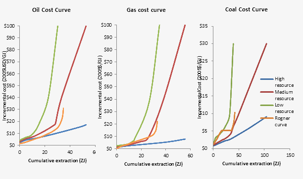
The parameters of the availability curves implemented as n-th order polynomials \(fp_{f,n}(p_f(t)))\) vary according to the type of fuel \(f\) and region \(n\). The following figure shows the global supply curves for which each a High, Medium, and Low case have been specified. By default, the Medium variant is used in the WITCH model.
By definition, we assume that cumulative extraction is equal to zero in 2005. In order to replicate observed data in the base year, we impose regional cumulative extraction in 2010 to be equal to the amount of actual production in 2005 multiplied by the time step (embedded in the parametrisation of the availability curves).
Since polynomial functions can replicate realistic cumulative production patterns only for a confined range of values, after 2100 we assume constant regional extraction shares.
\[ prodpp(f,t,n)= \sum_{n} Q_f(t,n) \times \left(\frac{prodpp(f,'20',n)}{\sum_{n} prodpp(f,'20',n)}\right) \forall t > 20 \]
While GHG emissions from Oil extraction are considered, see the previous section, emissions associated with the extraction of coal and gas are not considered.